SHAP Library Tools#
SHAP library has offers different visualizations. These are discussed here.
Dataset preprocessing, Model Training, Testing, Evaluation Metrics
Global Explanation Plots
Local Explanation Plots
1. Dataset preprocessing, Model Training, Testing, Evaluation Metrics#
# Uncomment the libraries not installed
#!pip install numpy
#!pip install matplotlib
#!pip install pandas
#!pip install scikit-learn
#!pip install xgboost
#!pip install shap
import numpy as np
import matplotlib.pyplot as plt
import pandas as pd
from sklearn import metrics

from sklearn.preprocessing import LabelEncoder
from sklearn.model_selection import train_test_split
from sklearn.preprocessing import StandardScaler
import xgboost as xgb
import shap
shap.plots.initjs()

drop_list = ['symmetry_worst', 'area_worst', 'symmetry_se','radius_mean','concave points_worst',
            'compactness_se', 'concavity_se','smoothness_se','perimeter_mean','concave points_mean',
            'texture_se','radius_se','smoothness_mean','texture_mean','concave points_se',
            'area_mean','compactness_mean','perimeter_worst','Unnamed: 32', 'id']
#importing our cancer dataset
dataset = pd.read_csv('data.csv')
dataset = dataset.drop(drop_list, axis = 1)
X = dataset.drop(['diagnosis'], axis = 1)
Y = dataset['diagnosis']
#Encoding categorical data values
labelencoder_Y = LabelEncoder()
Y = labelencoder_Y.fit_transform(Y)
X_train, X_test, Y_train, Y_test = train_test_split(X, Y, test_size = 0.25, random_state = 0)
sc = StandardScaler()
X_train_scaled = sc.fit_transform(X_train)
X_test_scaled = sc.transform(X_test)
classifier = xgb.XGBClassifier()
classifier.fit(X_train_scaled, Y_train)
Y_pred = classifier.predict(X_test_scaled)
print(metrics.classification_report(Y_test, Y_pred))
print(metrics.confusion_matrix(Y_test, Y_pred))
              precision    recall  f1-score   support

           0       0.99      0.97      0.98        90
           1       0.95      0.98      0.96        53

    accuracy                           0.97       143
   macro avg       0.97      0.97      0.97       143
weighted avg       0.97      0.97      0.97       143

[[87  3]
 [ 1 52]]
# set feature names to classifier
classifier.feature_names = list(X.columns.values)
2. Global Explanation Plots#
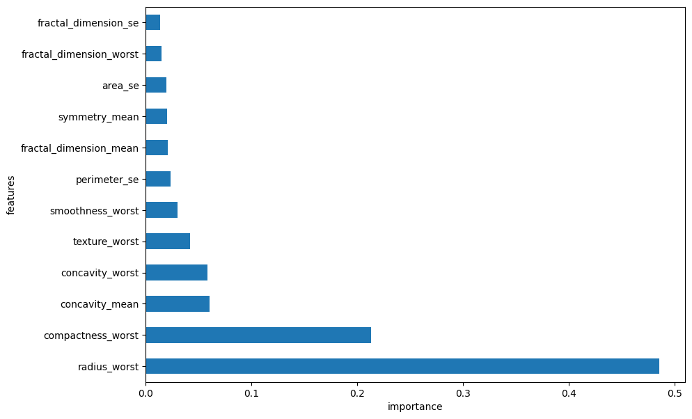
i. Global Feature Importance Plot#
plt.figure(figsize=(10,7))
feat_importances = pd.Series(classifier.feature_importances_, index=X.columns)
feature_importances = pd.Series((classifier.feature_importances_ / sum(classifier.feature_importances_)), index=X.columns)
feature_importances.nlargest(20).plot(kind='barh')
plt.xlabel("importance")
plt.ylabel("features")
Text(0, 0.5, 'features')
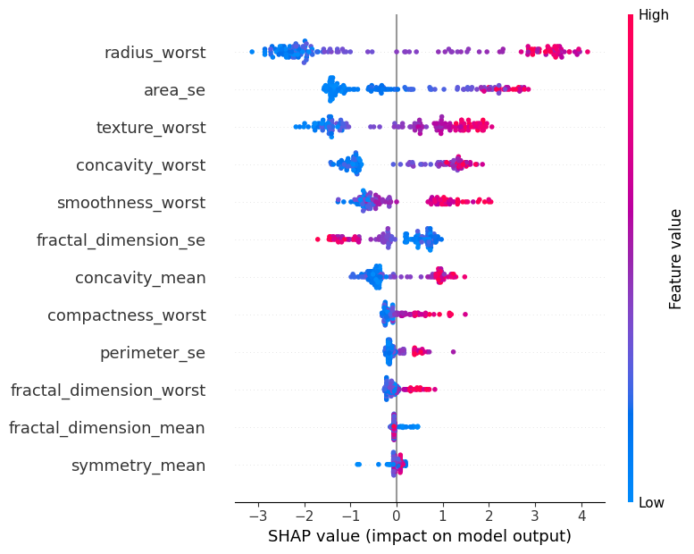
explainer = shap.Explainer(classifier, X_test_scaled)
shap_values = explainer(X_test_scaled)
shap.summary_plot(shap_values, X_test, feature_names=X.columns, show=False)

plt.show()
3. Local Explanation Plots#
i. Force Plot#
row_to_show = 5
data_for_prediction = X_test.iloc[row_to_show]  # use 1 row of data here. Could use multiple rows if desired
data_for_prediction_array = np.array(X_test.iloc[row_to_show]).reshape(1, -1)

# Create object that can calculate shap values
explainer = shap.TreeExplainer(classifier)
# Calculate Shap values
shap_values = explainer.shap_values(data_for_prediction_array)

shap.force_plot(explainer.expected_value, shap_values[0], data_for_prediction, matplotlib=True)
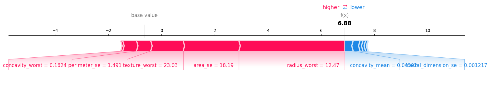
print("model prediction in log-odds space: ", np.log(classifier.predict_proba(data_for_prediction_array)[0][1] / classifier.predict_proba(data_for_prediction_array)[0][0]))
model prediction in log-odds space: 6.882191