SHAP and SHAPIQ Comparison Notebook#
I want to compare the shap library and shapiq library outputs, to check they provide the consistent results for some instances.#
The first section contains training the model, testing the model and evaluation metrics.
The second section contains choosing a data point for explaining from the test split.
The visualizations are plotted using both the libraries.
Question.
1. Data Preprocessing, Model Training, Testing and Evaluation Metrics#
# Uncomment the libraries not installed
#!pip install numpy
#!pip install matplotlib
#!pip install pandas
#!pip install scikit-learn
#!pip install xgboost
#!pip install shap
#!pip install shapiq
import numpy as np
import matplotlib.pyplot as plt
import pandas as pd
from sklearn import metrics

from sklearn.preprocessing import LabelEncoder
from sklearn.model_selection import train_test_split
from sklearn.preprocessing import StandardScaler
import xgboost as xgb
#import joblib
import shap
shap.initjs()

import shapiq
from tqdm.asyncio import tqdm

import warnings
warnings.simplefilter(action='ignore', category=FutureWarning)

drop_list = ['symmetry_worst', 'area_worst', 'symmetry_se','radius_mean','concave points_worst',
            'compactness_se', 'concavity_se','smoothness_se','perimeter_mean','concave points_mean',
            'texture_se','radius_se','smoothness_mean','texture_mean','concave points_se',
            'area_mean','compactness_mean','perimeter_worst','Unnamed: 32', 'id']
#importing our cancer dataset
dataset = pd.read_csv('data.csv')
dataset = dataset.drop(drop_list, axis = 1)
X = dataset.drop(['diagnosis'], axis = 1)
Y = dataset['diagnosis']
#Encoding categorical data values
labelencoder_Y = LabelEncoder()
Y = labelencoder_Y.fit_transform(Y)
X_train, X_test, Y_train, Y_test = train_test_split(X, Y, test_size = 0.25, random_state = 0)
sc = StandardScaler()
X_train_scaled = sc.fit_transform(X_train)
X_test_scaled = sc.transform(X_test)
classifier = xgb.XGBClassifier()
classifier.fit(X_train_scaled, Y_train)
Y_pred = classifier.predict(X_test_scaled)
print(metrics.classification_report(Y_test, Y_pred))
print(metrics.confusion_matrix(Y_test, Y_pred))
              precision    recall  f1-score   support

           0       0.99      0.97      0.98        90
           1       0.95      0.98      0.96        53

    accuracy                           0.97       143
   macro avg       0.97      0.97      0.97       143
weighted avg       0.97      0.97      0.97       143

[[87  3]
 [ 1 52]]
# set feature names to classifier
classifier.feature_names = list(X.columns.values)
2. Selecting instance from the test dataset to explain#
(change the instance id in the last row of this code block and run all the blocks below to see the results)#
def explain_instance(classifier, X_test, X_test_scaled, Y_test, instance_id):
    """
    Prints and returns the actual values, scaled values, and prediction for a selected instance.

    Parameters:
        classifier  : Trained model with feature names
        X_test      : DataFrame of test features (actual values)
        X_test_scaled : Scaled version of X_test (numpy array)
        Y_test      : True labels for the test set
        instance_id : Index of the instance to be explained

    Returns:
        dict: Contains actual values, scaled values, true label, and predicted value
    """
    x_explain_actual = X_test.iloc[instance_id]
    x_explain_scaled = X_test_scaled[instance_id]
    y_true = Y_test[instance_id]
    y_pred = classifier.predict(x_explain_scaled.reshape(1, -1))[0]

    # Print formatted output
    print(f"\n{'Feature Name':<25}{'Actual Value':<15}{'Scaled Value':<15}")
    print("=" * 50)
    for i, feature in enumerate(classifier.feature_names):
        print(f"{feature:<25}{x_explain_actual[i]:<15}{x_explain_scaled[i]:<15.4f}")

    print("\n" + "=" * 50)
    print(f"Instance ID     : {instance_id}")
    print(f"True Value      : {y_true}")
    print(f"Predicted Value : {y_pred}")
    print("=" * 50)

    return {
        "actual_values": x_explain_actual.to_dict(),
        "scaled_values": x_explain_scaled,
        "true_label": y_true,
        "predicted_label": y_pred
    }
explain_this_record = explain_instance(classifier=classifier, X_test=X_test, X_test_scaled=X_test_scaled, Y_test=Y_test, instance_id=0)
Feature Name             Actual Value   Scaled Value
==================================================
concavity_mean           0.1445         0.7121
symmetry_mean            0.2116         1.1253
fractal_dimension_mean   0.07325        1.5536
perimeter_se             3.093          0.1224
area_se                  33.67          -0.1450
fractal_dimension_se     0.004005       0.1112
radius_worst             16.41          0.0191
texture_worst            29.66          0.6640
smoothness_worst         0.1574         1.0870
compactness_worst        0.3856         0.8751
concavity_worst          0.5106         1.2170
fractal_dimension_worst  0.1109         1.5393

==================================================
Instance ID     : 0
True Value      : 1
Predicted Value : 1
==================================================
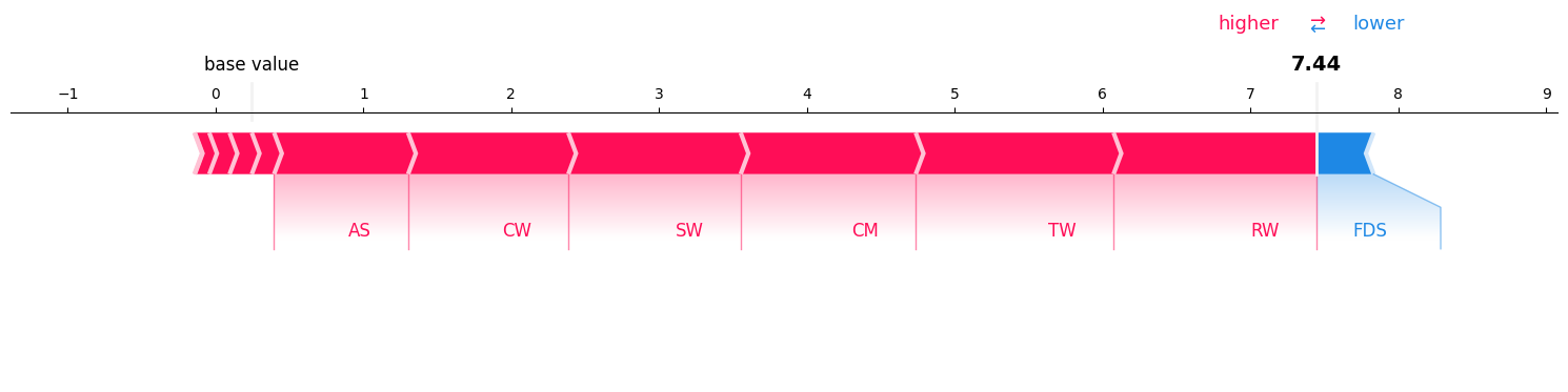
SHAPIQ#
Compute and Visualize the Shapley Interactions for that specific instance#
%%capture
# create explanations for different orders
si_order: dict[int, shapiq.InteractionValues] = {}
for order in tqdm([1, 2, len(classifier.feature_names)]):
    index = "k-SII" if order > 1 else "SV"  # will also be set automatically by the explainer
    explainer = shapiq.Explainer(model=classifier, max_order=order, index=index)
    si_order[order] = explainer.explain(x=explain_this_record['scaled_values'])
si_order
sv = si_order[1]  # get the SV
si = si_order[2]  # get the 2-SII
mi = si_order[len(classifier.feature_names)]  # get the Moebius transform

sv.plot_force(feature_names=classifier.feature_names, show=True)
#si.plot_force(feature_names=classifier.feature_names, show=True)
#mi.plot_force(feature_names=classifier.feature_names, show=True)
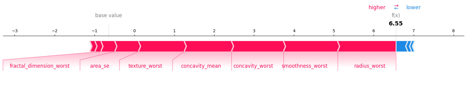
SHAP#
Compute Shapley Values for that specific instance#
data_for_prediction_scaled = pd.DataFrame([explain_this_record['scaled_values']], columns=X_test.columns)

# Create object that can calculate shap values
explainer = shap.TreeExplainer(classifier)
#explainer = shap.Explainer(classifier, X_train_scaled)
# Calculate Shap values
shap_values = explainer.shap_values(data_for_prediction_scaled)
print("shap values: ", shap_values)
print("base value: ", explainer.expected_value)
shap values:  [[ 1.1844642   0.1501946  -0.07178954 -0.09607071  0.59316266 -0.3014957
   1.4617031   1.1465104   1.3552241   0.12591067  1.3031968   0.3481194 ]]
base value:  -0.6462273
Visualizing the Model Explanation of the same datapoint using Shap#
shap.force_plot(explainer.expected_value, shap_values, feature_names=classifier.feature_names, matplotlib=True)
Comparison of the Numerical Outputs from both the libraries#
# Compute SHAP values using both explainers
shap_explainer = shap.TreeExplainer(classifier, X_train_scaled)
shapiq_explainer = shapiq.TreeExplainer(classifier, max_order=1, index="SV")

shap_values = shap_explainer.shap_values(explain_this_record['scaled_values'].reshape(1, -1))
print("shap_values: ", shap_values)
shapiq_values = shapiq_explainer.explain(explain_this_record['scaled_values']).values
print("shapiq_values: ", shapiq_values)

# Add baseline (expected value)
shap_sum = shap_explainer.expected_value + shap_values.sum()
shapiq_sum = shapiq_values.sum()#shapiq_explainer.baseline_value + shapiq_values.sum()

y_predict_proba = classifier.predict_proba(explain_this_record['scaled_values'].reshape(1, -1))[0]

print(f"True Label: {explain_this_record['true_label']}")
print(f"Predicted Label: {explain_this_record['predicted_label']}")
print("predicted probability: ", y_predict_proba)
print("Model output in log-odds:", np.log(y_predict_proba[1] / y_predict_proba[0]))
print("Sum of SHAP values + expected value (SHAP Library):", shap_sum)
print("Sum of SHAP values + baseline (SHAPIQ Library):", shapiq_sum)
shap_values:  [[ 1.14575763  0.16148624 -0.04058166 -0.07827457  0.78053839 -0.21634792
   1.57991888  1.43837674  1.23957111  0.13830555  1.5681721   0.43228585]]
shapiq_values:  [ 1.18446409  0.09737997 -0.38939594  1.37007074  1.33825598  0.00339744
  0.15092493  0.15019461  0.90652817  1.16593348  1.08382003  0.13755617
  0.24535655]
True Label: 1
Predicted Label: 1
predicted probability:  [0.00142395 0.99857605]
Model output in log-odds: 6.552892
Sum of SHAP values + expected value (SHAP Library): 6.552902340042975
Sum of SHAP values + baseline (SHAPIQ Library): 7.4444862226993695